
Time Series Classification through Shapelets Transform primitive
Let's explore how we can use Shapelets to perform Time Series classification. After an introductory, theorical, part, a practical example will be examined and addressed through the Python's library aeon.
Time series data are found everywhere, from temperature readings and stock prices to heart rate monitors down to website traffic logs. These streams of data, generated over time, contain very valuable patterns and trends that could be the key to many insights in various fields. However, this kind of data can be quite tricky to analyze and interpret because it is dynamic and temporal. That is where time series classification comes in. This technique enables a wide range of applications by labelling time series data with its inherent pattern, behavior, or characteristic. Be it the diagnosis of a medical condition from patient health data, the prediction of equipment failure in industries, or the detection of anomalies in financial transactions, the ability to classify time series data with accuracy is changing industries.
In today’s article we will look at a relatively recent primitive introduced to classify more efficiently time series belonging to different classes: the shapelets.
Theory
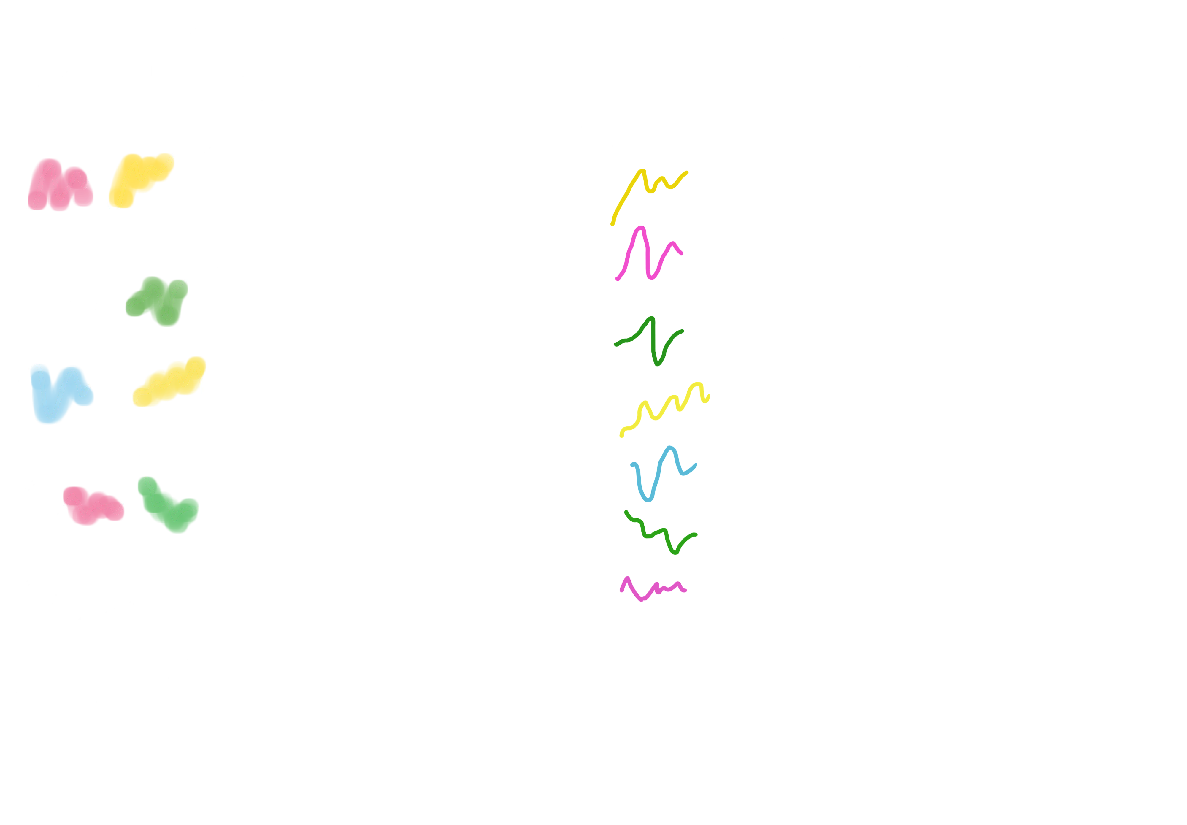
We can define a shapelet as a sub-sequence of a known time-series that is maximally representative of its class, i.e., that is characteristic of the class to which the time-series belongs. Let’s look for example at the image below: we have four different time-series, with the top-left and bottom-right ones belonging to class 1, while the others two belonging to class 0. The orange-highlighted sub-sequences could be potential shapelets that an algorithm can exploit to learn how to discriminate between the two different classes. It has been immediately interesting to me how the concept of finding shapelets is very near to how a human would behave in trying to understanding the differences between two sequences.

Among the various advantages that this primitive brought, I would like to focus on two precise issues that prove the robustness and the potential of the shapelets technique. First of all, learning or discovering a shapelet would mean to learn or discover a sub-sequence that characterizes an event, hence we are discovering new interpretable insights about our original time-series. That is not always the case: more than often, machine learning methods tend to work on compressed representations of the input data, hiding all the intermediate transformations performed during the analysis of the observations. Another strength is their robustness due to the local approach they have. Previous techniques were based on algorithms like K-NN and distance measurements to evaluate the similarity between two time-series. First of all, due to their dynamical and noisy nature, various and complicated distance measures have been developed trying to build more reliable estimators of similarity (see Dynamic Time Warping). However, even with those advanced metrics, global rumors that could affect the signal would inevitably distort the measurement, sometimes making the algorithm go off-track. In contrast, shapelets techniques work on local regions of the time-series, automatically ignoring corrupted sections of the sequence that do not bring any insights into labelling our data.
But how shapelets are found?
Now that we are clear about what shapelets are and why they can be very useful for our purpose, it is worth to have at least an idea on how those special sub-sequences are searched and extracted from the original time-series dataset. Different approaches have been developed during time, but all of them can be summarized in a two-step procedure:
- Candidate generation, i.e., iteratively extract all (or at least a good amount of) the possible sub-sequences from the input series.
- Shapelets evaluation, i.e., selection of the best candidates based on how they’re able to discriminate our input data with respect to their true labels.
Regarding the extraction of the candidates, those are extracted through sliding windows of sizes contained in a user-specified range. The boundaries of this range can be set both from a domain-knowledge point of view or with the help of model selection techniques like cross-validation and similar. For example, if we are analyzing ECG time series data, could be worth to set a minimum size equals to the average length of a single peak (that often is investigated to discover potential QRS complex alterations) while as maximum one a multiple of this minimum size, ensuring to capture subsequent peaks that could characterize bradycardic or tachycardic rhythms. Once this range is defined, for each time-series in the dataset, for each available size in the range, all the sub-sequences across the signals are extracted and listed as candidate (in practice, though, different algorithms exploits smart pruning strategies to avoid generating an unfeasible number of candidates).
After a pool of candidates has been extracted, it is time to evaluate each one of them to understand what is the best one in discriminating the current input data. Now, different algorithms have been developed to exploit the shapelets idea, each one with different characteristics. For example, the first approach to the shapelets was strictly related to the construction of a precise classification model, i.e. a Decision Tree, where, at each node, the best shapelet is chosen to be responsible in dictating the next split (based on how it is able to discriminate between the two classes of the current partitioned-data, exploiting the notion of information gain). Other approaches, like the one that we will use during the practical example (see the section below), try to find the best k shapelets from the whole pool of candidates (evaluating them against the whole dataset, differently from the Decision Tree approach), exploiting them to transform the task from a sequential to a tabular one. Obviously, different approaches require slight different techniques to compute the quality of a shapelet, but all of them rely on the following idea. First of all, we need to define a new measurement criterion for this quality, that we will call shapelet distance. Now, given a shapelet candidate and a single time-series, to find this shapelet distance we need to slide the candidate over all the sequence, computing for each window the euclidian (point-to-point) distance. Among those, there will be a window’s position that resulted in the smaller distance measure: this will be the best matching position of the shapelet to the time-series, and the distance value the shapelet distance. Now, let’s think about two time-series, with each of them belonging to a different class. A good candidate would results in two very different shapelet distances (usually one is very small, while the other significantly higher), hence allowing for the chance of discriminating between the two. Let’s see, for example, two candidates that are very different in terms of explaining the variances between two example time-series.
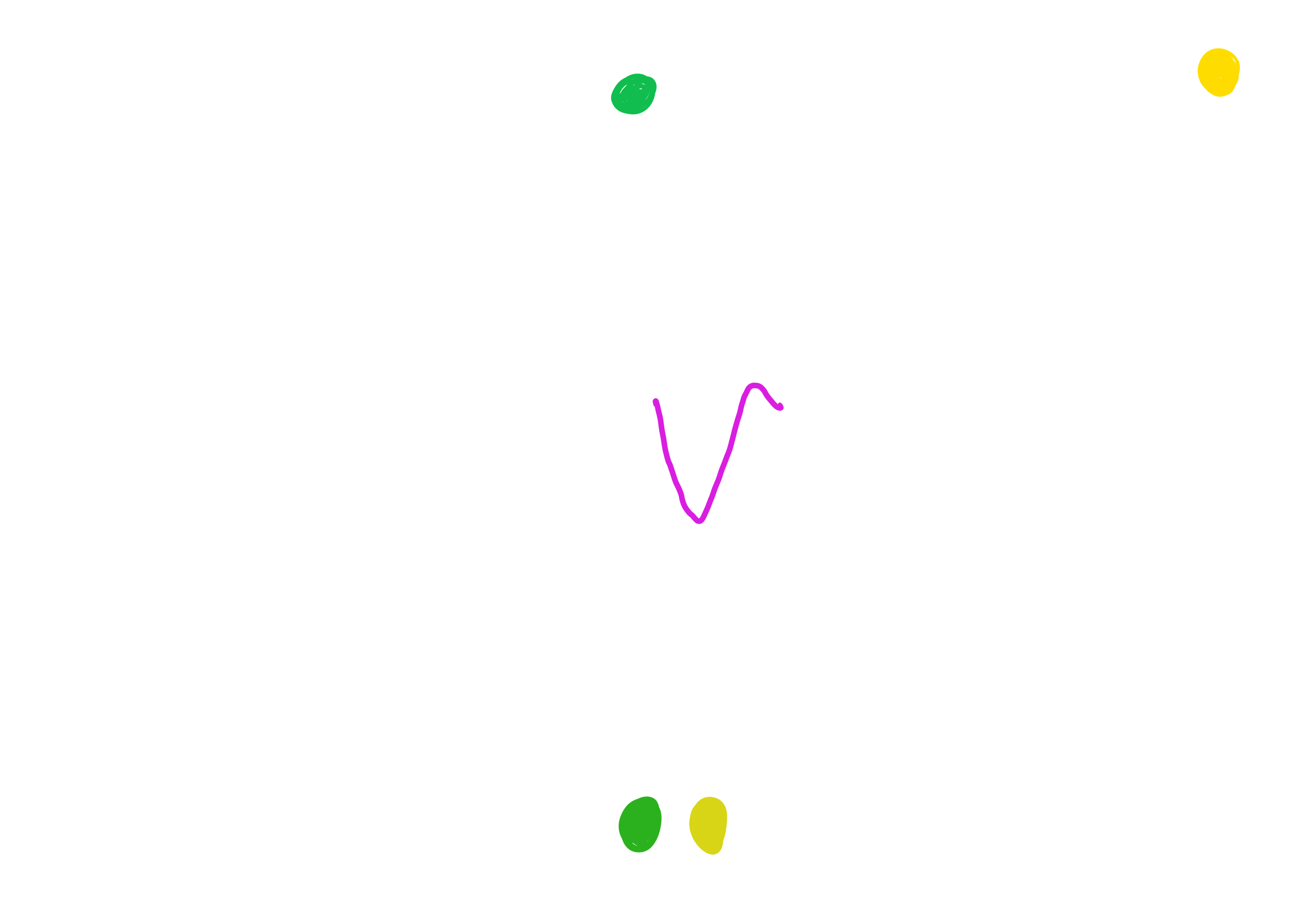
It is immediately noticeable how the pattern captured by the purple candidate is present in both the time-series. This will result in two shapelet distances that are not so different. The best matching overlap is pretty good on both the time-series, hence the distances will be both relatively low (or still similar).
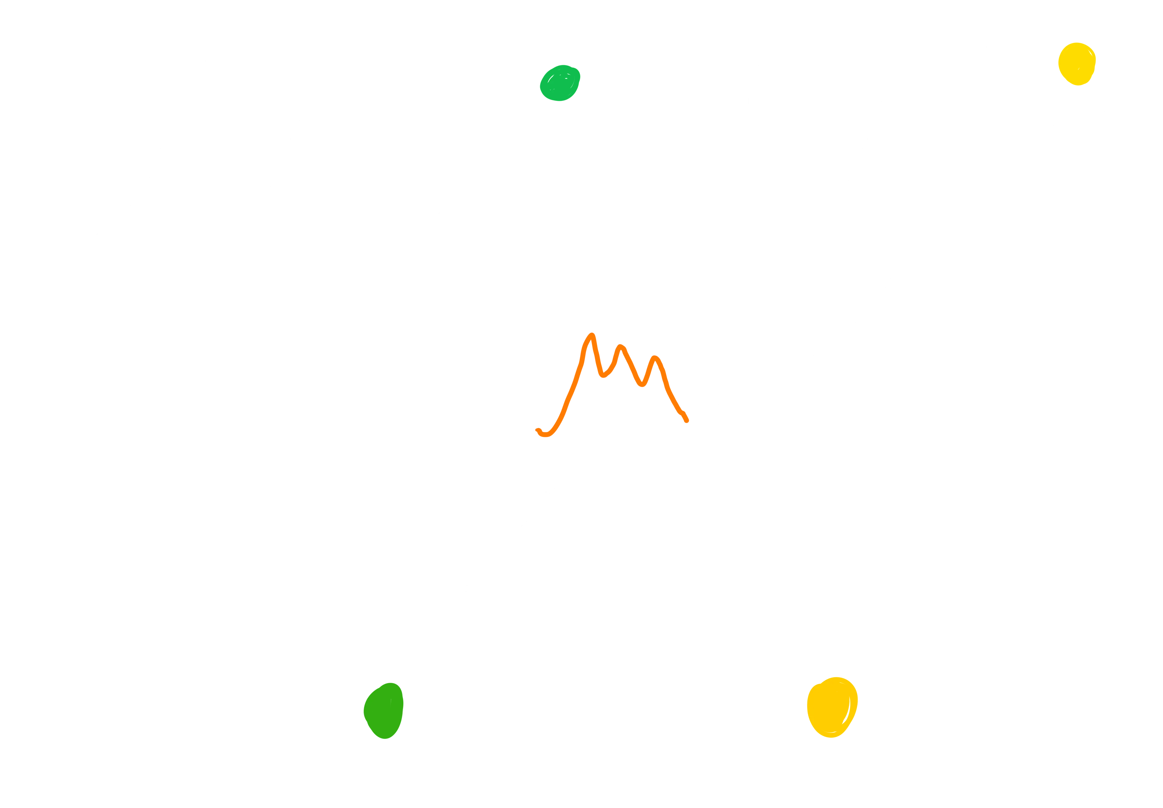
On the other hand, the orange one seems to be a particular pattern that is contained only in the green time-series, hence the minimum distance between the shapelet and the yellow one is significantly higher than the minimum distance from the green one, resulting in a better division of the two samples.
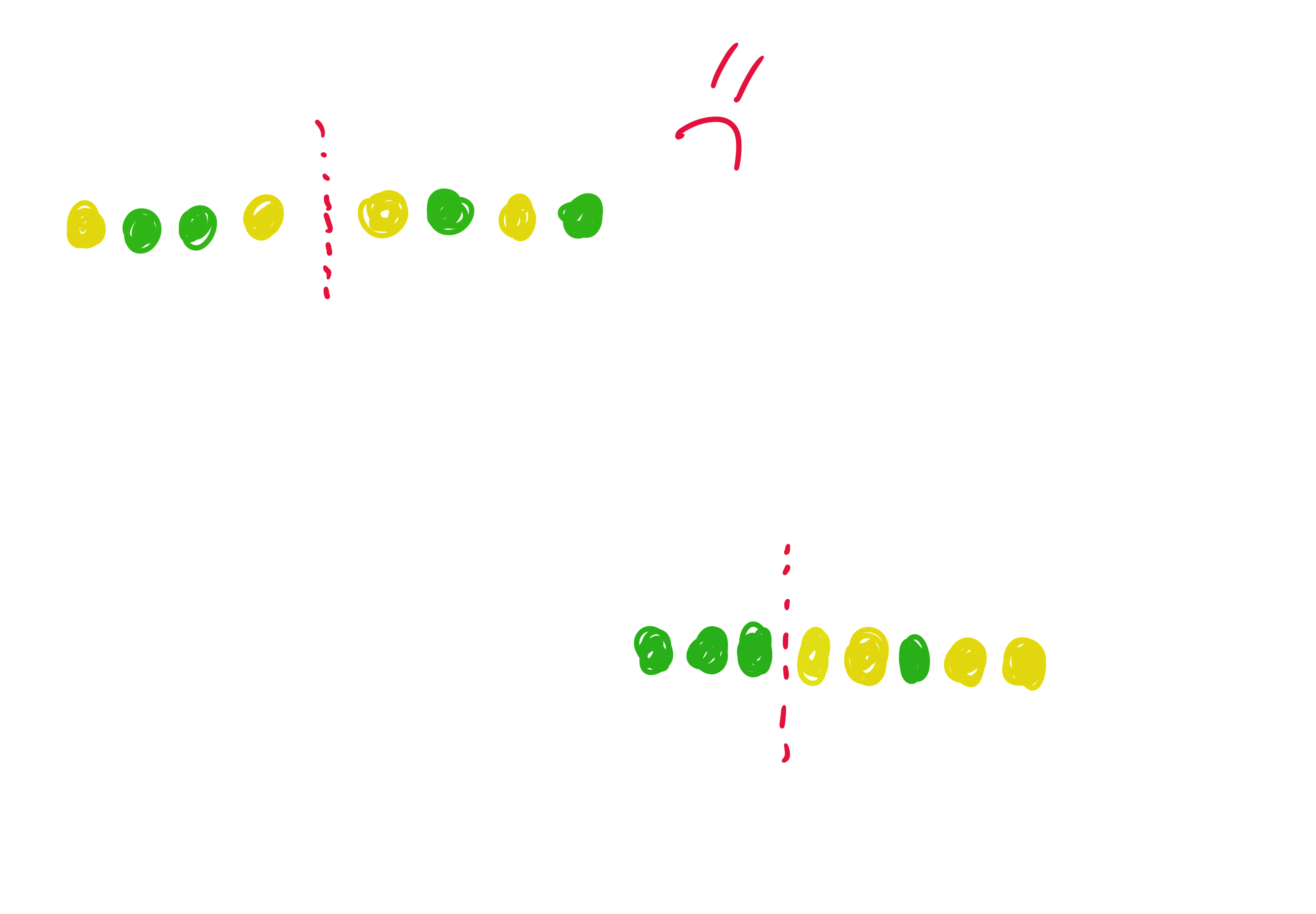
At this point, the best candidate, is the one that (ideally!!!) is able to place all the distances computed upon all the time-series dataaset on the imaginary axis (depicted in the two previous figures) in a way that the split between the classes is maximized (i.e., concept of information gain).
As we already said, cleary the real algorithms are more complex than this, with different approaches exploited in searching the shapelets through a lot of optimized solutions that improve the efficiency of the search. However, what we have seen by now should be enough to have a rough idea of what are we dealing with in the next section.
Practical Example
To explore the subject in a more practical way, we will try to see how the shapelets perform on a well-known dataset, defined as a binary classification task where a movement of pointing a real gun should be discriminated from a fake pointing with just the index finger. I will use the Python library aeon in a Google Colab notebook. The method provided by the aeon library is a slight modification with respect to the first shapelets-approach, recognized as shapelet transform. First of all, a new hyper-parameter k is requested here: from the whole pool of candidates, the best k shapelets will be searched and selected as the shapelets to use. The idea is that once the time-series are exploited to find our best k discriminative sub-sequences, the original signals are discarded and mapped into a new input space, where each observation is composed by the distances (defined as the shapelet distance explained in the previous section) from the old time-series to each of the best k candidates. Please note that even if the original time-series are discarded, the insights gained while searching the shapelets is preserved (i.e., it’s still possible to visualize the shapelets).
Let’s formalize a little bit: given a set of n time-series defined as follows:
and given the best k shapelets retrieved from X (or better, from the pool candidates):
the new input of our classification task will be defined as follows:
Okay, that should be enough to have an idea of what is happening here. Coming back into our notebook, let’s visualize the signals divided by the different classes to discover some patterns that could be captured by our shapelets.
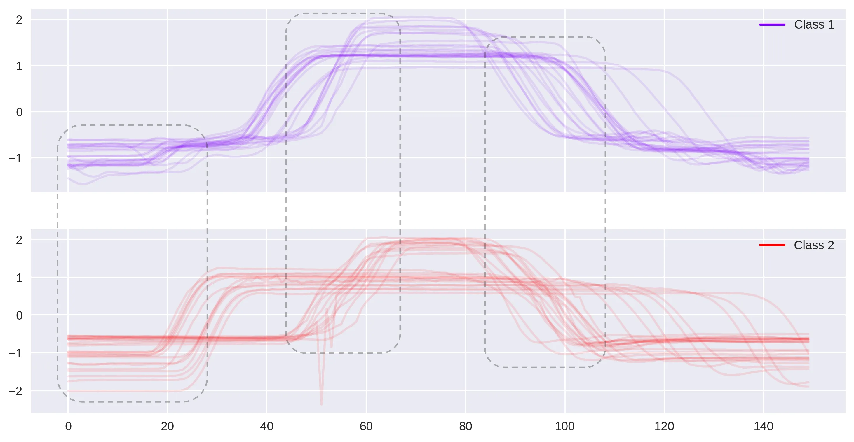
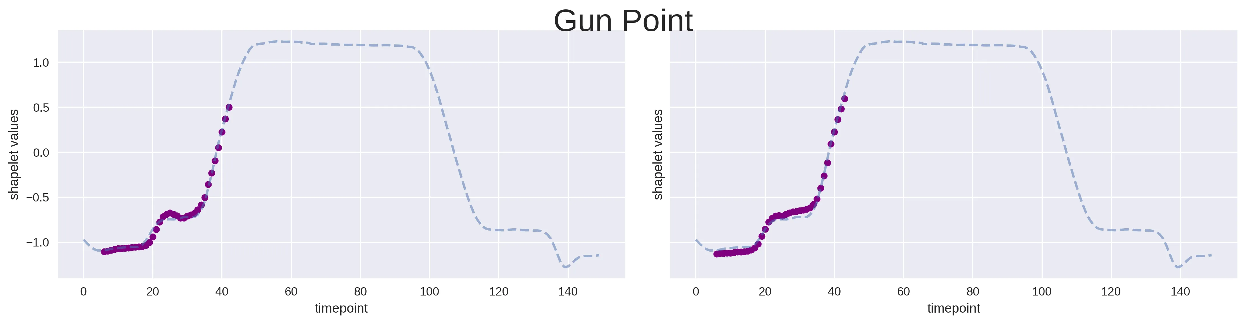
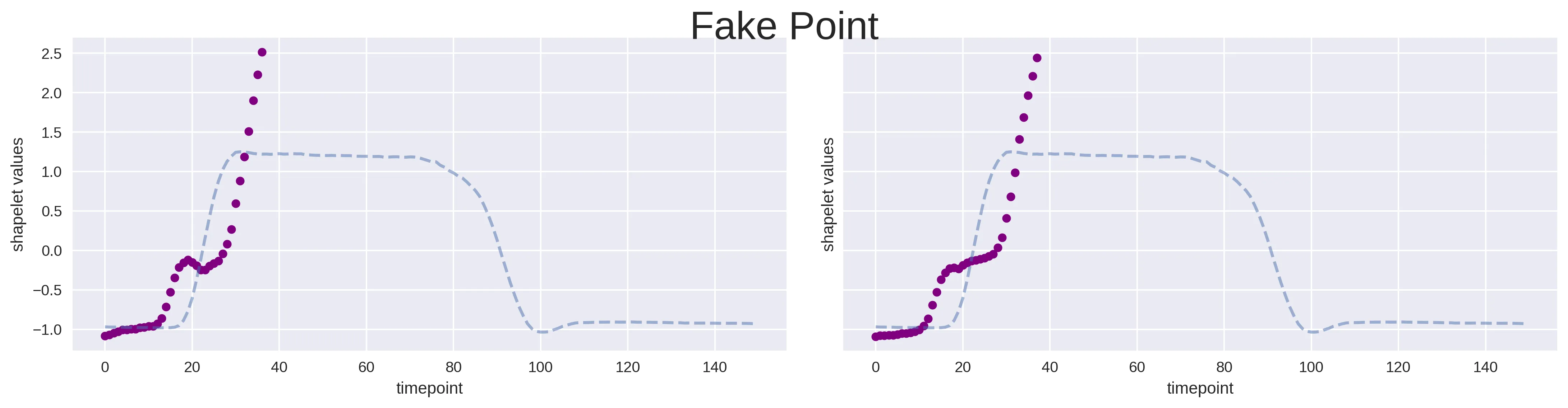
As you can see, there are some sections where the time-series from different classes seems to behave in a very characteristic way, hopefully guiding the search of our candidates. From this initial naked-eye analysis, we can also deduce good ranges within which to set the search for candidates. For example, could be worth to try something like 20 as the mininum shapelet size, while 40 for the maximum, a range where all the major differences seems to lie. This will also speed-up the search of the candidates with respect to leaving the algorithm without any hint of this kind. At this point, the search of the eight best shapelets (i.e. k = 8) has been run. Down below it is possible to see two of them overlapped in their best matching position against a time-series from both classes: it is clearly visible how those two shapelets are very good in discriminating the sequences from class 1 (gun point) with respect to the other ones (fake point).
Among the advantages of this transformative approach, there is the chance at this point to use whatever classification model we like. A good idea would be to perform a model selection in which different of them are evaluated against each other, to discover the one that would perform better. Now, given that the scope of this article is focused on the shapelets understanding, I just tried a Random Forest classifier, fitted with the best hyper-parameters found performing a grid-search cross-validation. The obtained results are listed below:
| Class | Precision | Recall | F1 |
|---|---|---|---|
| Gun Point | 0.97 | 0.99 | 0.98 |
| Fake Point | 0.99 | 0.97 | 0.98 |
| Macro Avg | 0.98 | 0.98 | 0.98 |
It is important to note, that the test set should be transformed too through the shapelet-transform agent, remembering that this has been fitted only on the training set (i.e., the shapelets are extracted only from the training set). As we can see, even if we discarded the time-series in favor of a tabular representation, the shapelets were able to provide a modified input that was great in capturing the discrimination between the two classes, as indicated by the great result of 0.98 for the F1-Score 🥳.
📚 References
- Time Series Shapelets: A New Primitive for Data Mining
- A shapelet transform for time series classification