Problem-Solving AI Agents

I started studying, again. October marked my new beginning at University of Pisa, as a student of the AI curriculum for the Computer Science Master's degree. I decided to begin from the Artificial Intelligence Fundamentals course which goal is to give us the fundamentals of the AI discipline. Starting from the definition of a rational agent, we will dive in into the concepts of reasoning, planning and solving problems, searching for solutions to them.

One of the first issues that an AI practicioner has to face is to understand and define as clearly as possible the environment of its problem. There are some framework that helps to standardize that definition, but you can easily imagine what are the main aspects to take attention to. One of those is the knowledge of the environment upon which the problem relies. For example, would be great to predict the presence of a disease from a simple blood analysis, and that's the case for some of them. But there are certainly some disease for which we didn't found yet a systematic correlation between values and prediction. In those cases, technologies like AI comes in help. That was an example in which there is a lack of knowledge, but you can also be faced with a real lack of visibility: let's think of a maze for example, or maybe a robot that wants to clean your house. It does not know the house "structure" before making an exploration phase. So, as you can imagine, there are a lot of possibilities here, both from the environment point of view, both from the instruments that you have to choose while addressing the problem.

The concepts in that course start to look at those problems relaxing the real-world scenarios, investigating abstract and simplified environment first. So, let's imagine ourselves in a fully observable environment. That means that in every moment, we are able to have a complete point of view upon the whole problem, aware of all the information that we need to solve it. At the same time, though, we also know that we are not able to immediately tell with certainty what's the correct action to take to reach our goal. With that environment in front of us, the correct instrument to use are the so called problem-solving agent, which strategy is to plan ahead and consider a path that bring them from a starting point toward the goal state. That process is known (by all of us) as search.

Let's give us an example problem now: we are a little funny cell of a grid. We know that this grid has a maze, and we also know that we want to find our friend, that is somewhere inside the grid. Lastly, thanks to our drone, we also have a clear view from the top of the grid that gives us the whole knowledge of the current situation of our environment.

First thing to do, we have to formalize the problem as a search problem:

• What are the states on which the environment can be in? Defining the state space, we can say that it is composed by the set of the grid's cell coordinates.
• What's the initial state? It's where we are right know, the coordinates of our position in the grid.
• What is the goal? Is there only one of it? We have to find our friend, so our goal will be the coordinates of our friend in the grid.
• What are the actions that we can take? Well, generally speaking we can go ahead toward the top, right, bottom or left cell. In that case, we should be careful to not step on the walls of our maze, though.
• What is the effect of our action on the environment? Also called the transition model, it serves us to explain what is the state resulting from a certain action taken from a certain state. We know this, we just need to update our coordinates based on the direction of the movement.
• What is the cost of our actions? For example, let's imagine a navigator agent. We need to know how much kilometers is long every available roads towards our goal to minimize the costs for our passenger (actually, maybe would be worth to focus on the time, but it's just an example).

Okay, we should have everything now to solve our problem. As we already said we need to find the correct sequence of actions that brings the agent from the initial state to the goal state. The agent will find it building a search tree where:

• the root of the tree is the initial state;
• on every state, the agent will consider all the legal actions that can be taken from that state (we formalized this information before) and will take them, expanding the current node to create different branches of the tree;
• all the current leaves node, form the so-called frontier, i.e. the list of nodes that can be expanded in the subsequent search step. Which node will be chosen by the agent from the frontier is what characterizes the chosen searching algorithm. This is one of the most important choice to make when designing the agent;
• when a node is chosen from the frontier for the expansion, the agent will check if that node encodes the goal state. If so, the search is ended and the problem's solved!

Let's bring that theory to a practical example. Supposing we have a 3x4 grid, with a starting and a goal position well defined.

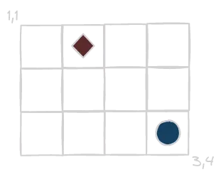
So, as you can see the initial state is (3,4) while our goal is (1,2). At the beginning of the searching process, our frontier will be made out of only the initial state.

• Choose a node from the frontier. How? Let's just randomize this choice right know, we will later see different strategies that we can adopt in that step. Anyway, at the beginning we will have only one choice: the initial state.
• Is this a goal state? Nope, so we have to take the actions phase.
• What are the legal actions that we can take from the current state? In this particular case, we are in (3,4) so we can only go up and toward the left.
• Taking all the available actions, we will expand the tree and put those resulting nodes (obtained by adding 1 to the right coordinate, as described by our transition model) in our frontier;
• New iteration!

When a goal state is found, we just need to backtrack using the parent property to build all the way up the solution path.

I have made up an image that could help us to grasp a bit more around the search loop described above, let's see and discuss it.

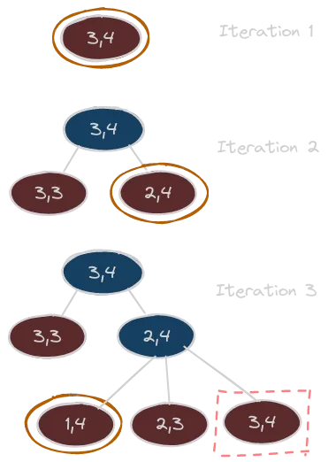
I feel like we need a legend here, so, at each iteration:

• the red nodes are the ones contained in the frontier;
• the blue nodes are the ones that have been already chosen and expanded;
• the orange outlined nodes are the one chosen from the frontier for the expansion;

You can also notice that there is a node outlined by a dashed red boxy rectangle. Looking at it, we can see that it seems to be a duplicate. Actually, it's not so right to use that duplicate word: we said that those nodes contains more information outside of the simple state that they encodes, like the cost of the path, the parent and so on. So, even if the encoded state is the same as the root, the nodes are pretty different! Anyway, it was important to highlight this possible situation, because could be part of the design process to implement some kind of strategy to avoid redundant paths like this one. Actually, there are some cases where this is a necessary choice to avoid infinite loop. My advice would be to always implement a strategy to avoid redundant path. The simplest way to do that would be to keep track of the visited state and avoid expansion that bring us again on those already checked. There are some cases, though, were this decision can be a little bit too greedy! That's because can happen that a path that we see as redundant maybe bring us to the same state with a better performance measure (i.e., with a lower cost). So, would be wise to keep track of the visited node, but also to check against them taking into account the cost spent to arrive there.

Great, so know we know the whole theory that we need, and we also understood that there are actually two main aspects in that search framework just presented:

• the strategy used to choice the node to expand from the frontier;
• the strategy used to check for redundant paths during the search process;

These two things characterize the different search algorithms, that we can divide into two main categories:

• Uninformed search: the family of algorithms that does not exploit knowledge about what is known about the goal during the search process;
• Informed Search: the family of algorithms that exploit that knowledge to improve the quality of their search. With quality, we means maximize the performance measure of the agent (e.g., minimize time when using our Google Maps application).

Uninformed Search

Breadth-First search (BFS)

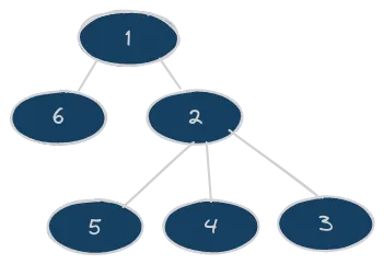
The idea of this algorithm is to explore broadly the search tree, checking all the nodes at a certain depth before going down on the tree. I labeled in that graphic the order in which the nodes would be visited by this algorithm:

From a practical point of view, this is implemented treating the frontier as a FIFO queue (for example, using the shift array method of Javascript when retrieving, assuming the use of push when inserting). Every time we want to expand a node, we have to choose the oldest one in the frontier. Talking about the strategy of checking against already visited nodes, we just need to check for the encoded state, without taking care of comparing the cost between the old and the redundant node. This is because, as per its nature, the Breadth First search algorithm ensure us that every time we visit a node, this has been visited through the optimal way (i.e., with the best performance measure).

Depth-First search (DFS)

Differently, as its name suggests, DFS algorithm tries to go as deep as possible before trying other branching routes. Again, here is a little graphic labeled to show you the order of visited nodes:

From a practical point of view, this is implemented treating the frontier as a LIFO queue (for example, using the pop array method of Javascript when retrieving, assuming the use of push when inserting). The idea is to expand always the last inserted node, the youngest one. Different is the issue with redundant paths here. First of all, it is extremely important to implement one, because this algorithm is very vulnerable to infinite loops. There is another issue, though: differently from the Breadth First search, DFS does not ensure us to find the optimal solution. For that reason, is really suggested to implement that redundant strategy not only checking against the state encoded in the node, but also using the current cost of the already visited state. Maybe that redundant path is better!

Dijkstra's algorithm

We are now moving over something that prove more reasoning. DFS and BFS have inside them a lot of mechanical-nature. They are systematic, and they face a great challenge when the state space is huge. We should start to think smarter, introducing a little bit of (artificial) intelligence. The Dijkstra's algorithm is still an uninformed algorithm, but at least it tries to exploit what it can knows about the environment: the frontier management strategy is to choose the node with the lower path cost (up to that moment). Now, let's make up another example with respect to the simple grid. That's because in the grid example every action has the same cost, so it's not so helpful to visualize the nature of this algorithm. Inspired from the AIMA example of Romanian roads, let's imagine this situation:

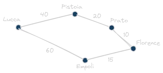
We are in Florence, and we want to reach the city of Lucca, following the instructions given by the Dijkstra's algorithm. The numbers on the arches are the costs of the roads (they are random, they don't recall the reality). That's the reasoning done by the algorithm:

• at the beginning we just have Florence in our frontier, let's expand it;
• we have two nodes in the frontier: Empoli, with a cost of 15, and Prato, with a cost of 10. The algorithm will choose the cheaper one: Prato! Expanding it, we put in the frontier Pistoia, with a cost of 30;
• we have two nodes in the frontier: Empoli, with a cost of 15, and Pistoia, with a cost of 30. Empoli is chosen and expanded. Now we have Lucca in the frontier, with a cost of 75. It is important to notice that, even though Lucca is our goal, we are not stopping here. That's because we can still find some better paths to it.
• we have two nodes in the frontier: Lucca, with a cost of 75, and Pistoia, with a cost of 30. Expanding Pistoia, we are ready for our last step!
• we have two nodes in the frontier: Lucca, with a cost of 75, and Lucca with a cost of 70. The chosen solution will then be Florence-Prato-Pistoia-Lucca one!

We have just experienced an interesting property of this algorithm. Even though we found a goal state earlier, we waited on labeling it as a solution, cause as long as we have some path with a lower cost, we could have potential solutions that are better!

Informed Search

Before presenting two of the most famous informed search algorithms, we need to define the meaning of that informed definition. The main idea is that the agent will exploit some kind of information about the goal state. This information is called heuristic. Defined as a function of the current node n, we can say that h(n) is the estimated cost from the node n toward our goal state. Now, there is a bunch of theory around those concepts, especially to prove optimality of some algorithms based on the heuristic's nature. By now, let's just assume those requirements for our heuristic function:

• the heuristic function is always greater than 0;
• the heuristic function of a goal state is equal to 0;
• the heuristic function of a node is always less or equal to the real optimal cost from that node to a goal state (i.e., the heuristic function is literally an optimistic estimation);

Now we can take a look at the two algorithms.

Greedy best-first search

The idea here is to choose from the frontier the nodes with lower heuristic value first. It seems to be reasonable: we know that the heuristic is an estimation of the real optimal cost, so, we prefer to focus on those nodes that seems to cost less toward our solution. Actually, this is not so straight-forward, and we can see why with an example. Then, we'll have pretty clear the reason of the greedy definition. Let's imagine this strange, but possible, situation:

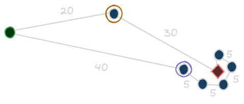
First thing first, we should define our heuristic. For sake of simplicity, let's say that h(n) is the straight-line distance between the state n and the goal state (i.e., the red diamond). Okay now, supposing that our initial state is the green filled circle, the greedy approach will rather choose the state outlined by the purple circle with respect to the orange one. From there, it will follow the chain of states so close to the goal. If you sum the path cost, though, you can see that this path is worse than the other one. It is clear indeed what is the issue with that algorithm: it relies only on the estimation of the heuristic, without taking care of the actual cost needed to follow the current route.

A* Algorithm

To approach this limitation, the A* algorithm comes in our help. Its idea is to take into account, when choosing the node to expand, not only the value of the heuristic, but also the real cost to reach the node (it combines them computing the sum of those when evaluating nodes). Intuitively, we can understand that this algorithm will try to minimize the estimated cost to reach the goal while minimizing the actual cost of the solution path. This makes the A* algorithm not only complete, but also optimal (with the requirements that we put on our heuristic before). Recalling the previous example:

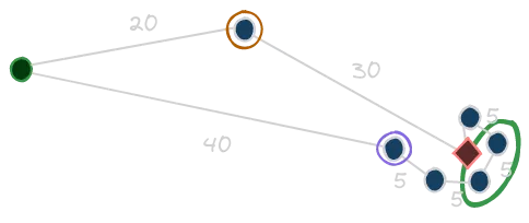
With respect to the path followed by the greedy approach, with the A* algorithm there will be a moment where the cost of the sub-optimal route will make the whole evaluation function greater with respect to the other one. This moment will be more or less around the nodes that I outlined with the light green ellipse. It is there that the A* will switch to the other path, finding the one that is actually optimal!

Introducing Searchy 🔎

If you have read my previous article, you already know that I don't like theory without practice. The goal of this article was to consolidate to myself the understanding of those concepts, as they are part of the program of my University's course. But while studying them, I thought would be cool to implement and visualize them from a concrete point of view. That is why I'm introducing to you my little side-project 🔎 Searchy .

🔎 Searchy wants to be an environment to test and visualize different problem-solving AI agents (i.e., searching algorithms) upon a simple problem as a fully-observable maze scenario. You can see a glance of it in that screenshot:

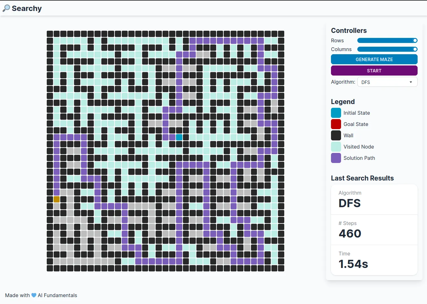
Right know, the usage is pretty simple: you have a grid, and you can customize the number of rows and columns. You can generate a randomized maze and the chosen algorithm will perform the search. Once the search is started, a couple of stats will be gathered during the process. Those are finally shown in the result section in the sidebar, together with the solution path on the grid.

My willingness is to open source this and try to continuously improve and evolve it to support less trivial scenarios, more algorithms, more insightful performance comparisons and so on. Would be good to have this application as a robust environment on which try, understand and test searching algorithms while studying those concepts.

📚 References

• Artificial Intelligence: a Modern Approach

💻 Practical References:

• Searchy 🔎