Genetic Algorithms: exploring 3D object reconstruction

In the previous article, we talked about how an AI agent can find its way to solve a problem with the usage of searching techniques. We had a fully observable environment, with a clear and fixed objective: reach the goal. The question that we gave to the agent was: how can I reach the goal (in an optimal way) given your starting position and the environment around you?

However, we are not always interested about the path towards a goal. Sometimes, we only care about the goal itself. Let me clarify this with an example: suppose that you have a couple of commitments during the week. You want to build an agent that, given the list of commitments (with potential day/time constraints), will build a schedule that helps you organize your crazy week. Now, you can imagine how we are not interested in stuffs like: okay I try to put this event in that moment. Then the other one there, and so on... We don't care, we just want the final snapshot of our organized week. Our solution is not a path towards our organized week, it's just our filled week.

This is the key concept that characterizes another kind of problems in which AI agents can successfully being applied: Optimization Problems. The goal of the AI agent is to find the state that maximizes some kind of performance measurement. Even if pretty different, the problems are approached in a similar way from the AI agent: with a search. The searching strategy used to solve optimization problems is called local search, because the agent will start from a starting state, and evolves it in the local neighborhood trying to improve it.

Different techniques exist to address those kind of problems, with one of those being Genetic Algorithms, a tool explicitly inspired by the natural selection theory.

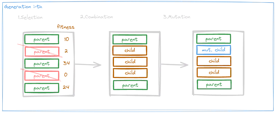
Let's formalize it. We said that our aim is to find the state that optimize a performance measure, that we will call here fitness function. The main idea, is to start out generating an arbitrary number of random initial states, called out population. Now, every state of the current population is evaluated with respect to the fitness function, implicitly rating and assigning them a goodness value. The best ones are then selected, and combined to give birth to the next generation. From time to time, can happen that some of those offspring are affected by random mutation. This process is then iterated until we find some state that maximize our fitness function, giving us a solution or a great approximation of it.

Intuitively, we can imagine how each random generated initial state allows us to cover a wide part of the space-state (which can be pretty huge for this kind of problems). Then, the combination of those narrows the search-space that we are investigating during time, hopefully toward the section of it where our solution lies. Finally the mutations helps us to avoid or escape any local maxima or plateaus that characterizes the space-state of those problems.

One of the most interesting aspect of Genetic Algorithms, in my opinion, is the huge customizable nature that they offers: every one of those phases just described above, are fully left to the design process, opening a lot of opportunities of explorations and improvements. Now we'll see a couple of standard examples for each of those phases and then going to try a practical example of application of genetic algorithms.

Theory

Requirements

While approaching an optimization problem with genetic algorithms, the first thing to do is to represent the problem itself in a way that suit the algorithm's nature. That's probably the most crucial phase and is highly dependent on the problem's domain. The focus should be put into two issues:

• How we will represent each individual in our population? Typically, each individual is represented by a string of character over a defined alphabet. The go-to example is about using binary strings (we will use this for our examples in the next sub-sections). One example where this representation is suitable could be the knapsack problem: you have a list of item, each one with a value and a weight. Then you have a knapsack, with a maximum weight capacity. The goal is to maximize the value of the items in the knapsack without exceeding the weight. In this case, you can encode the individual as a binary string where 1 means inserting the respective item in the knapsack, while 0 means the opposite. Different is the scenario of the Traveling Salesman Problem (TSP). This is one of the most famous optimization problems in theoretical Computer Science, that involves finding the shortest possible route that visits a set of cities exactly once and returns to the origin city. In that case a binary representation could be improved with an integer-string one. For example, given the cities 1, 2, 3, ..., n , we could represent an individual as a string of integer that indicates the order of visit of the cities. The hard truth, though, is that the most of the real-world problems lies on a continuous solution space, requiring an individual representation as a real-valued vectors (e.g., [0.2, 3.2, 1.2]). The most trivial example is the function optimization problem.
• How we will evaluate each individual in our population? What is our fitness function? This is another domain-related choice. If you think, for example, at the function optimization problem, it is natural to use the function itself as the fitness one. Sometimes, we need to use an heuristic, because the ideal fitness function is not known. Let's think for example about the knapsack problem: we could define the fitness function with respect to the sum of the items values and a penalty term growing as the weight exceed the capacity. The only limit is imagination here. Anyway, the fitness value will be computed, in every phase of the evolution, for each individual in the current generation. That is crucial, because the next step will be strictly related to the fitness values: the selection phase.

Selection

The selection phase aims to select those promising individuals that will be in charge of developing the next generation. The how of this step is defined in the combination phase. Usually, the selection is probability-based, and the probability of an individual being picked is strictly related to its fitness value, encouraging the selection of the more promising ones. Let's see a couple of strategies:

Roulette Wheel Selection

The main idea is to iteratively select a parent with a probability directly proportionate to its fitness value. The idea is to attach a probability of selection to each individual, directly computed from its fitness value with respect to the sum of all the fitness values.

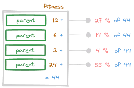
Rank-Based Selection

This strategy is similar to the Roulette Wheel Selection method, with a slight difference. Previously, the probability of being picked was computed directly from the fitness value. In this new method, however, the fitness value is used to sort, or rank, each individual. From there, the probability for each individual is computed as the percentage of its position with respect to the sum of the total ranks. Let's clarify this with a picture.

With respect to the Roulette Wheel Selection, we can see this method as a little bit more fair towards the worst individuals. The better one are more likely to be chosen, but the difference in percentage is not directly related to the difference in fitness value.

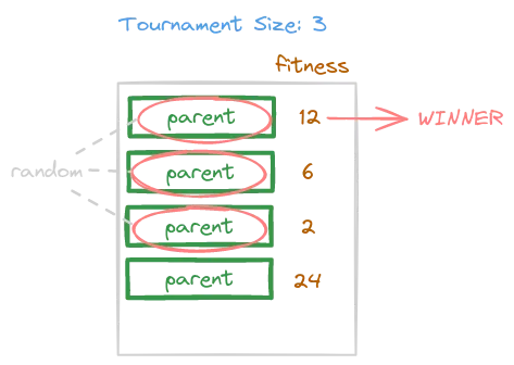
Tournament Selection

The idea here is to select in a uniform random way two or more individuals. From that batch of individuals the best one in terms of fitness value will be selected. The number of randomly picked inviduals is called tournament size, and it's an hyper-parameter of this strategy.

Combination

With the combination phase, a newer and (hopefully) more promising generation of individuals is created from the selected parents. This step wants to be an analogy of the sexual reproduction in biology: the idea is to transfer into a new child some informations from both the parents. Now, unlike the previous steps, this phase is a little bit more dependent from the representation chosen for each invidiual. Let's start exploring some techniques assuming binary string individuals.

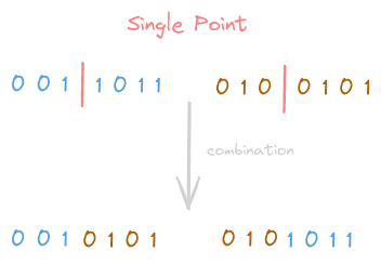
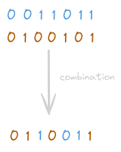
Single-Point Crossover

Initially, a combination location is chosen from both the parents (the same location will applied to both). From that situation, two children are generated, swapping the two parts of each parent into each of the new children.

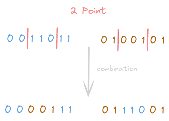
K-Point Crossover

This is a generalization of the Single-Point Crossover. The point is to have multiple combination points (locations) useful to the swapping procedure. Below a picture showing a 2-point crossover.

Uniform Crossover

The previous two methods take whole portion of the parents and exchange them, transferring information to the children. In the uniform approach, the gene of a new child is determined independently, choosing randomly between one of the two genes of the parents. For example, the first bit of the first child, could be the first bit of the first parent with a certain probability x, or the first bit of the second parent with a certain probability y. The probability assigned to each parents is another design-choice (hyper-parameter? Based on fitness?).

Mutation

The mutation step consists in a small, randomized, change to a generated individual. It occurs based on a probability, usually set at a pretty low value: it can be harmful, especially if not set properly, moving the current individual far from the desired solution. However, optimization problems often presents a lot of traps in the search-space (shoulders, local-maxima/minima, ridge, etc...): the mutation step proves to be of fundamental importance to address those kind of problems, often escaping them successfully. The mutation operation is usually pretty simple, modifying one or a little number of gene of an individual. Let's look at some examples.

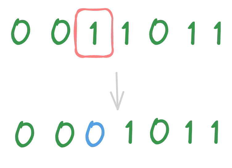
Flip Bit Mutation

The idea is to select a random gene of the individual and flip it (remember that this gene will be a bit).

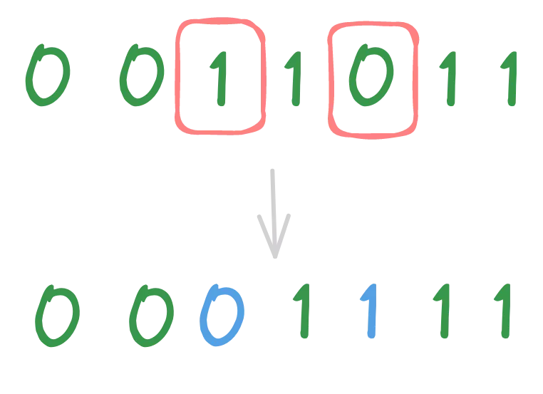
Swap Mutation

The idea is to select two random gene of the individual and swap them. Note that this operator can be applied even if the representation is not binary-based.

Real-Valued individuals

What we have just seen is an overview of genetic algorithms. We explored a couple of different strategies that can be used through all the algorithms' step to solve our problem, and we've done that assuming a binary-based or integer-based representation. As already said, though, the majority of real-world problems involve the need of real-valued based individuals. Now, regarding the selection phase, all the explored strategies are still valuable in case of real-valued individuals, which is not true for the stages of combination and mutation. Let's see the two most famous operators used in those cases, leaving it to the reader to search for the different techniques proposed over the time.

Simulated binary crossover (SBX)

The idea here is to replicate the benefits and properties of the crossover as applied on binary-based inviduals. One of those properties is the equality of the averages of parents and children. Please refer to the paper "Simulated Binary Crossover for Continuous Search Space (K. Deb, R. Agrawal)" to explore the theory behind this concept. We will see now the equations that rules the SBX combination operator:

where:

• the subscripts 1 and 2 encode the first and the second parents when applied to y. Furthermore, the subscript i encode the i-th coordinate of the vector.
• the β parameter is called spreading factor and it controls how far from the parents coordinates the resulting one will be.

Real Mutation

The idea is to replace a value (a single item of the vector) with a brand new value. Now, the first attempt could be to randomly generate the new value, but this could bring to a new individual that has no relationship with the old one, causing an harmful evolution. Better ideas is to use some heuristic to generate the new random number. The simplest strategy is the Gaussian mutation: the random number will be generated using a normal distribution with a mean value of zero and some predetermined standard deviation.

Hyper-parameters

There are some hyper-parameters involved in an evolution strategy:

• Number of generations to iterate: could be a fixed number or accompanied by an error tolerance to perform early-stopping if a satisfying solution is found. Another idea could be to iterate as long as the difference between the solutions of the last x iterations are not different enough (i.e., there is no more improvement over time).
• Probability with whom the mutation takes place.
• Probability with whom the combination takes place. If it does not occur, then the parent is carried to the next generation as it is. This is called elitism.
• Population size: how many individuals will be evolved?

Experiment

Time for some practice now. The idea is to try to design and apply a genetic algorithm to reconstruct a 3D object model starting from the array containing its vertices information. In its core, a 3D object model has three key pieces of information, which are the minimum essentials for visualizing the model:

• Vertices, that defines the position of the vertices of the object, i.e., its structure;
• Normals, that defines the behavior of lights and shadows on the model;
• Indexes, used to understand how the triangles that compose the mesh are organized;

All of those three items have the form of an array of real-valued numbers (actually, the indexes are integer-based values). Also, we will focus here only on the reconstruction of the vertices array: for the other two items, you just need to re-run the strategy to reconstruct them too.

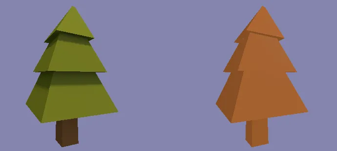
This is the base model that we will try to recreate. The implementation part will be done with the DEAP framwork.

First Attempt: Greedy Approach

First attempt: we know that the vertices are stored in an array of 360 real-valued numbers. So, let's try to run a genetic algorithm on it and see how it looks the reconstructed one. Let's follow the previous explained phases to design the algorithm:

Requirements

• The individuals will be represented by a vector of 360 real-valued numbers. We know as per domain-knowledge that those values are bounded in the range [-1, 1].
• Regarding the performance measure function, we need something that is able to tell us the distance between two arrays, the true one and the predicted one. Let's go with the Mean Absolute Error (MAE), that I prefer over the Mean Squared Error due to its robustness with respect to outliers. The MAE is expressed as below:

Selection

For the selection method, the tournament one has been chosen. With a k (number of individuals fighting with each other) equals to 3.

Combination

For the combination method, I used a particular version of the Simulated Binary Crossover (SBX) called Bounded SBX. The idea is to have the new individuals always bound in a pre-defined range. This is possible due to the domain-knowledge for which the vertices positions are always bounded in the range [-1, 1].

Mutation

The mutation phase follows the idea of the Gaussian one, using again a bounded variant.

Hyper-Parameters

The most interesting hyper-parameter here is the mutation rate. We said that our individuals are vectors of 360 items. That a pretty huge target to reconstruct. This large nature of our vectors bring us towards a pretty big search-space. To help us traverse this huge space, a relatively big mutation rate has been used (0.7)

This is the obtained result:

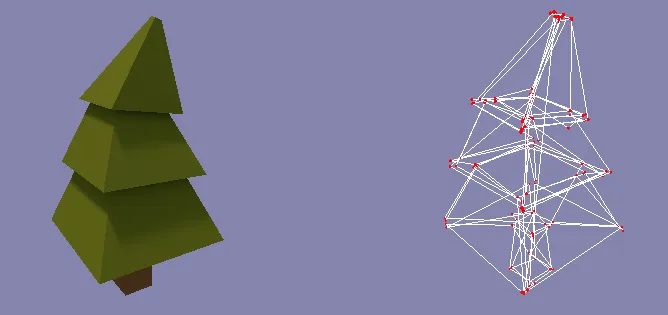
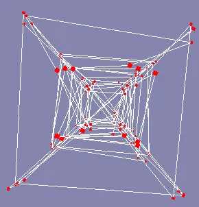
As you can see, the result is not so bad, but still a lot of turbolence is present. This issue is clearly visible while viewing the model from a bottom point of view:

Let's try a (hopefully) better approach.

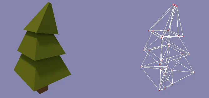
Second Attempt: Problem Decomposition

The problem’s approach proposed by genetic algorithms does not take into account notions like feature understanding, extraction or detection. There is no interpretation or learning of the structure to reconstruct, it is instead a systematic search towards a proposed solution guided by some heuristic function. On the other side, it could be useful to exploit not only the vertices position by themselves, but also the relationship between their position. A lot of powerful tools can be used to address this problems in a way that would take care of this aspect too, potentially enhancing the research process. Taking into account the fact that genetic algorithms do not fit into this set of tools, thought, we can conclude that zooming on the single vertices position can only improve the quality of our solution. The idea of this second strategy is indeed to deconstruct the problem, trying to run a different instance of the genetic algorithm for each vertex. From a practical point of view, in the context of our problem, that means switching from an attempt to reconstruct a vector of 360 elements to dealing with a couple of vectors of 3 elements each. Note that this approach opens up to the opportunity of parallelize the search process, drastically improving the execution time. Also, this search-space reduction allows us to follow a more stable search direction, lowering down the mutation rate value while improving the accuracy.

Here, the result:

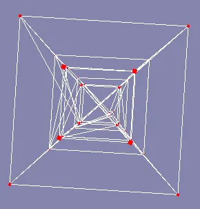
To complete the comparison, I want to provide the bottom point of view too:

Concluding, let's bring in the indexes array to correctly create the mesh triangles over the reconstructed structure:

Genetic Algorithms seems to work pretty good 🥳.

📚 References

• Artificial Intelligence: a Modern Approach
• Simulated Binary Crossover for Continuous Search Space (K. Deb, R. Agrawal)
• Analysing mutation schemes for real-parameter genetic algorithms (Kalyanmoy Deb and Debayan Deb)

💻 Practical References:

• Hands-On Genetic Algorithms with Python
• DEAP framwork