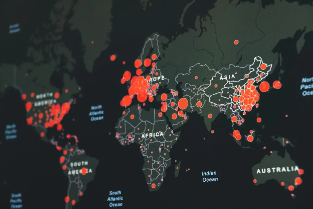
Agent-Based Models: Simulating an Epidemic

Theory

Complex systems

A system can be seen as a set of things working together as parts of a mechanism or an interconnecting network; a complex whole. More often than not, systems evolve by changing their state over time (both continuously or discretely). These kinds of systems are called dynamical systems. A particular class of dynamical systems is that of complex systems, where many simple components, or agents, interact with each other, causing a collective complex behaviour to emerge. Studying, observing, and understanding those systems could provide useful insights regarding the reachability of a state (predictions), behavioural patterns, or effects of perturbations of the system, generally allowing us to understand all the phenomena that happen around us in our everyday lives.

Computational Models

But what really takes to fully understand those kinds of systems? We need to build models, formally defined as follows:

Generally, models are expressed in terms of mathematical tools that represent the properties of the modelled system, while narrowing down the definition into the Computer Science world, we can then define what is a Computational Model.

Please note three key points of this definition:

• The focus is set only on the dynamical systems.
• A mathematical representation is necessary, due to its unambiguousness.
• The model must assume a computer-executable form, allowing for the computation of the system's evolution over time (e.g., performing a simulation).

Agent-Based Models

An agent-based model (ABM) is a computational model in which a system is modelled as a collective of agents that can make decisions, perform actions and interact with other agents and the environment they live in. Each agent is seen as an autonomous entity, usually characterized by a set of relatively simple properties and rules (often based on the agent locality). Making those interact with each other (usually through computer simulations) will allow for complex behaviour to emerge, enabling us to understand its properties and dynamics. Note how this definition goes along with the definition of a complex system. But why those models are very useful and somehow needed for us? Well, it’s because our world is getting more and more complicated. First, the systems we need to study and model are becoming more interconnected and complex. Old-school modelling tools just don’t cut it anymore. Second, some systems have always been too complex to model properly. Take economic markets, for instance. In the past, we had to assume things like perfect markets, everyone acting the same, and long-term balance just to make the math work. But now, with agent-based modelling, we can drop some of those unrealistic assumptions and get a much more accurate picture of how economies work. Third, we’re collecting way more detailed data these days. We have micro-level data that lets us simulate individual behaviours, which wasn’t possible before. And finally, the biggest reason: computers are getting way more powerful. We can now run huge, detailed simulations that would’ve been impossible just a few years ago. So, in short, agent-based modeling is taking off because it helps us tackle the complexity of today’s world in ways that older methods can’t.

From a practical perspective, the environment is typically modelled as a 2D or 3D space, often using a grid-based format. In this setup, each cell can be occupied by agents that move throughout the space to explore and exploit their surroundings. While exploring, agents can perform actions or interact with other individuals through simple pre-defined rules that we will call the Transition Function. The agents can be in a state among those defined by a set of available states. The specification of these dynamics defines the model on which we will base the simulation of the system under analysis. In the next section, we will introduce a JavaScript framework that can help in building and animating ABM simulations, showing how it works through a practical (and very simple) example.

AgentScript.js

AgentScript is an open-source library for writing ABMs. It is inspired by a programming language called NetLogo, probably the most famous tool to work with the agent-based simulations. Taking a look at the NetLogo's documentation, we can find the following words:

or,

It really seems to be what we need to exploit this modelling approach! 🤩

An AgentScript program (more precisely web application) can be composed of three major entities: a Model, a View and some Controllers (the framework has been built around the MVC architecture to clearly separate the components).

The Model is the definition of the system's approximation under study. From a code point of view, it's a JavaScript interface (hence must be extended by your custom model) that, in its simplest form, should be used as follows:

import Model from "https://code.agentscript.org/src/Model.js";
import World from "https://code.agentscript.org/src/World.js";

class MyModel extends Model {
  constructor(worldOptions = World.defaultOptions(50)) {
    super(worldOptions);
  }

  setup() {
    // your implementation here
  }

  step() {
    // your implementation here
  }
}

Starting from the constructor, we can see a parameter named worldOptions, defined from a static method of the World class: this is the class that helps us define the environment on which our agents will move around. Defined as a two or three dimensional grid, the World is mainly represented by the boundaries of the three coordinates:

WorldOptions = {
  minX: integer,
  maxX: integer,
  minY: integer,
  maxY: integer,
  minZ: integer,
  maxZ: integer,
};

At this point, we need to create life inside our world, i.e., create agents and the specifications that rule their behaviour. AgentScript provide three ingredients to fill the environment:

• patches: a patch is a single cell of the defined world, that is divided into a certain amount of equal-size squared cells. The patches cannot move, being static agents, but are able to be alive in terms of states;
• turtles: a turtle is an agent that moves around the world. Each turtle knows the patch it is on, and interacts with that and other patches, as well as other turtles. Turtles are also the end points of Links;
• links: a link is a connection between two turtles that could be used to create constraints or to abstract some kind of relationships;

A model, by default, will have those three members accessible from the beginning to start animating the world. Another important concept that is shared between all of those, is the one of the breed. A breed defines a special sub-type of an agent, that can be restricted to behave in a slightly different way. For example, let's consider two cells of our world, one representing the road and the other one a region of water. Those are both patches, but a turtle populating a road cell should behave differently with respect to another one in a water cell (or, changing the point of view, the same turtle upon the two different patches will have different consequences based on the patches rules). To summarise, we can usee breeds to set a kind property to our agents.

Regarding the model, that's it! Using all the ingredients just seen, we can implement the step and setup methods to replicate an approximation of our (complex) system. Note that this is enough to run simulations and perform analyses with their results (as long as you will call the setup method followed by as many step as you want).

But what if we want to see the current state of our simulation? We have to dive into the V of the MVC paradigm: AgentScript provides two different helper classes, TwoDraw and ThreeDraw, respectively specialized in drawing a 2D or a 3D world. Focusing only on 2D worlds right know, a TwoDraw instance can be used in its purest form as follows:

const model = new MyModel(worldOptions);
/**
 * To create the starting state of the simulation.
 * i.e., to have something to see!
 */
model.setup();

const view = new TwoDraw(model, viewOptions);

/*
 * I put them below just to clearly separate concepts and
 * better distinguish the different parameters of the
 * constructor.
 */
const viewOptions = {
  /**
   * The id of the div DOM element
   * where you want the canvas to be drawn.
   */
  div: "myDivId",
  /**
   * Dimension (forced) of the canvas. All the agents
   * will be scaled to respect those dimensions. Another
   * way of defining the canvas' size is by indicating the size
   * of a single square patch.
   */
  width: 500,
  height: 500,
  patchesColor: (patch) => {
    /**
     * Return the HEX string of the color that
     * that specific patch should have. Note that
     * from the object you can retrieve its state and
     * whatever you decided to store as a member.
     */
    return "#ff0000";
  },
  turtlesColor: (turtle) => {
    /**
     * Same as above, but for Turtles.
     */
    return "#00ff00";
  },
  // Size of a turtle in terms of patches fraction
  turtlesSize: 1,

  // and many other...
};

I left some comments on the code snippet to explain briefly some of the view options available. For an exhaustive list of properties and methods you can check directly on the source code here.

Now that the view is properly configured, we can invoke the draw method to depict the model's current state (i.e., the state it reached after the number of steps you've executed) onto a canvas injected inside the div provided in the configuration. Let's look at the below image for a moment:

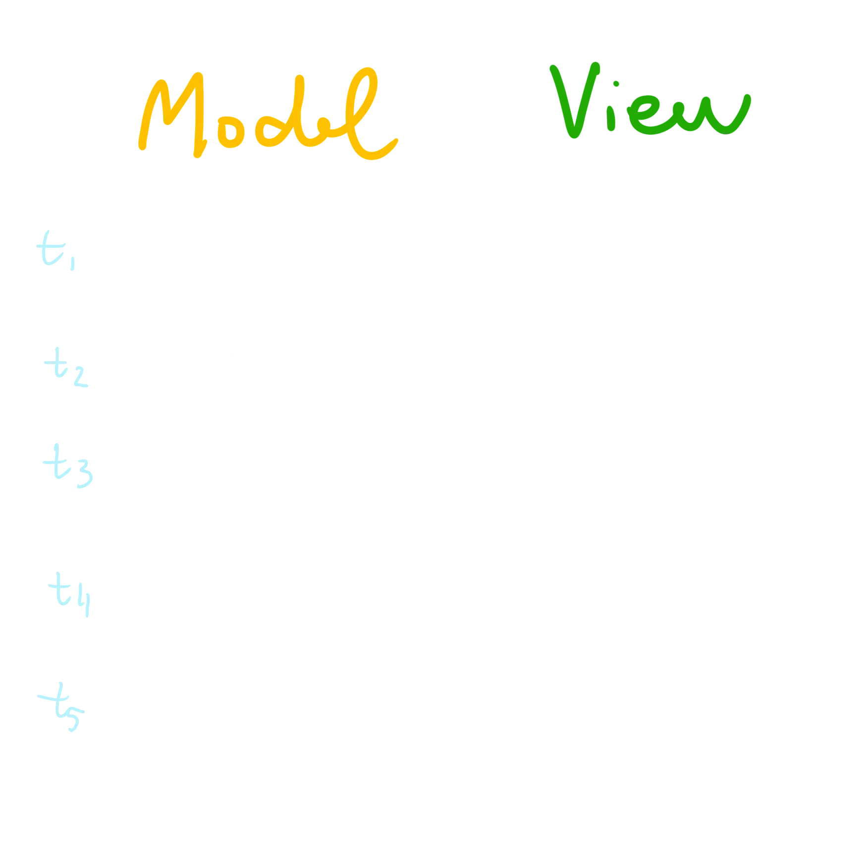
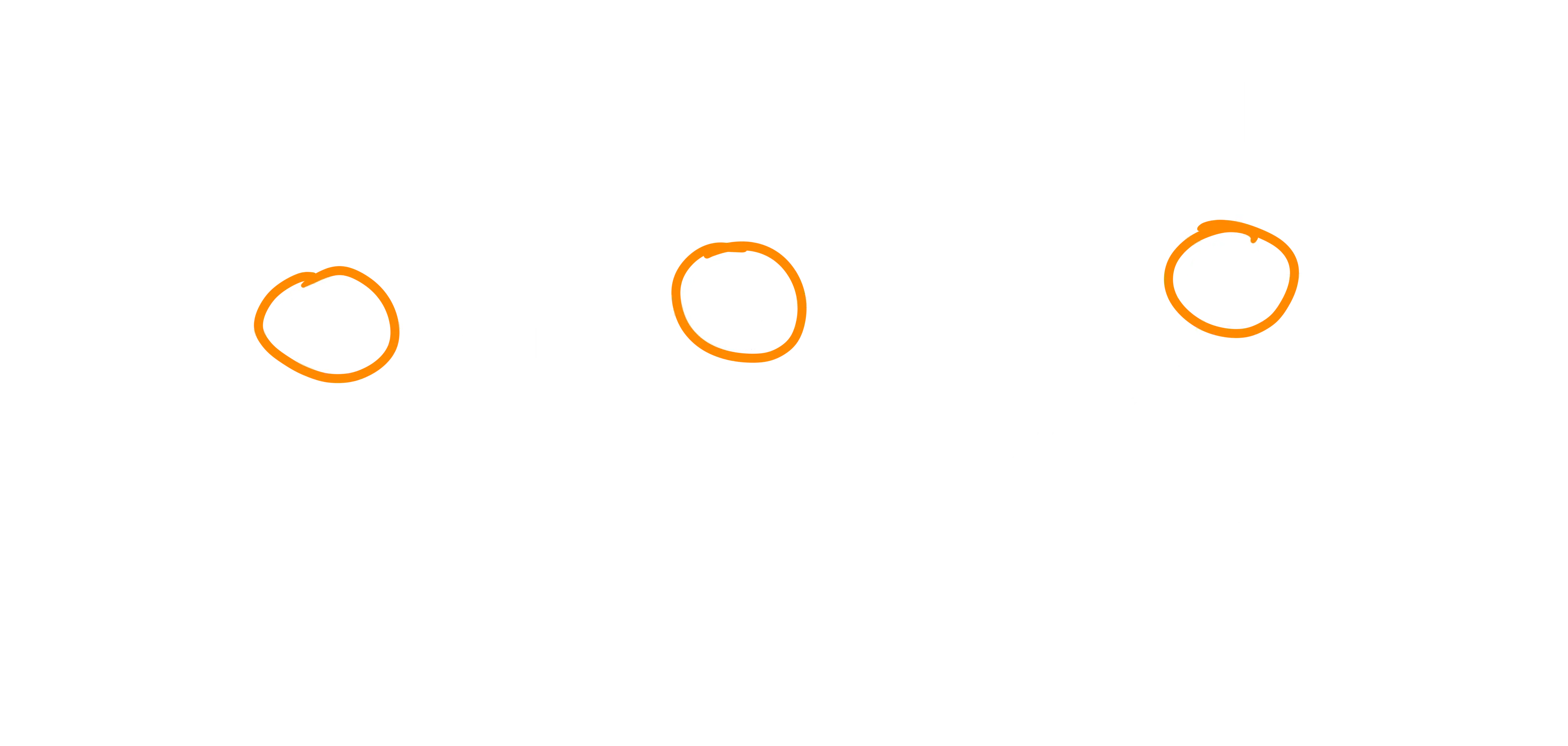
In the above scenario, the model would proceed for 4 steps in total, being drawn at t4. Note that the model's state at t5 would not have been depicted in this fictional example. Hence, it should be pretty easy to understand how we should use the two primitives (model and view) together: a first idea might be to implement a for loop that ensures that the call of the various steps is followed by a draw. If you're familiar with how JavaScript works, though, you will argue that this is not the best way to go:

• First of all, we are blocking the main thread. That is not a great choice, especially if the number of steps performed is high;
• Acting this way, we will not obtain any animation effects! The canvas will be updated so fast that the user will only see the final result.

The solution here is to use the setInterval API to schedule repeatedly calls to a provided callback with a fixed time delay between each call. Another choice would be to use the requestAnimationFrame method, a powerful animation primitive provided by JavaScript. However, we will stick with setInterval, since AgentScript uses this function. The use of setInterval allows for the customization of the update rate of the view, hence giving a chance to select the fps at which different images are drawn.

And so, we got to the C of the MVC as well. Among the different tools provided to control the simulation (e.g., a class that allows for the live-tuning of the model settings exploiting the dat.gui library) we can find the Animator, an abstraction that makes it possible to implement exactly the mechanism just described, starting from a desired number of fps (check this page to explore deeper the APIs).

Let's conclude this section with a practical example, where we are going to implement the famous Game of Life experiment with AgentScript. Firstly, we need to recall the model that defines the system (approximation):

• 🗺️ The world is a two-dimensional orthogonal grid of square cells.
• ☠️ Each cell can be in one of two possible states: live or dead.
• 🏘️ The neighbourhood on which the transition rules are based is Moore's one (i.e. eight neighbours: horizontally, vertically and diagonally adjacent).
• ⏭️ The transition rule is stated as follows:
  • Any live cell with fewer than two live neighbours dies, as if by underpopulation.
  • Any live cell with two or three live neighbours lives on to the next generation.
  • Any live cell with more than three live neighbours dies, as if by overpopulation.
  • Any dead cell with exactly three live neighbours becomes a live cell, as if by reproduction.

Let's address these points one at a time, implementing them as they go along.

• 🗺️ It's pretty straightforward: that is exactly how the World is defined in AgentScript. Hence, we only need to choose the size of our grid while defining the constructor of our custom Model.
• ☠️ This point leads us to an important observation: we've seen how AgentScript's world is populated by (among the others) turtles and patches. The former has been defined as moving agents, while the latter is the floor where the turtle moves. At the same time, though, the patches are also agents themselves, hence being labelled as static agents: in our example, we will not need to use any turtle, sticking only to the patches. The second portion of the issue is about the states that these cells can be in. This opens up another discussion: how can we handle the state of an agent in this framework? In the first place, each agent is a JavaScript object, allowing us to set arbitrary properties to save and stick values to a single entity. However, I'd rather use a specific mechanism provided by the framework, named breed. The idea is that it is possible to define sub-species of turtles or patches that share similar characteristics. For example, in this scenario, we could specify two different breeds, one to represent the living cells and the other one for the dead cells. Apart from the semantic meaning of the assigned breed, the usage of this API allows one to directly access the sub-set of interests without cycling over all the agents while checking on some property-value pair. Let's see some code:

// GameOfLifeModel.js

setup() {
  // Defining the available breeds for the patches
  this.patchBreeds("live dead");

  // Set pseudo-probabilistically the starting breeds
  this.patches.ask((p) => {
    p.setBreed(Math.random() < 0.1 ? this.live : this.dead);
  });
}

step() {
  /**
  * Here, I can use this.live directly to access
  * the sub-array of patches with breed 'live'.
  * The other option would force me to cycle/filter over
  * the whole patches array (less efficient).
  */
}

//

Note the usage of the ask method: it is just an abstraction upon the classical for cycle (with some checks upon agent's implicitly generated ids). You can think of it like a forEach method. For those who are interested, the abstraction is there to make sure that if you generate new agents of the same set in the ask callback, the cycle will only cover the old set and not the updated one (in a sense, it is to mantain atomicity of the step with respect to the original set).

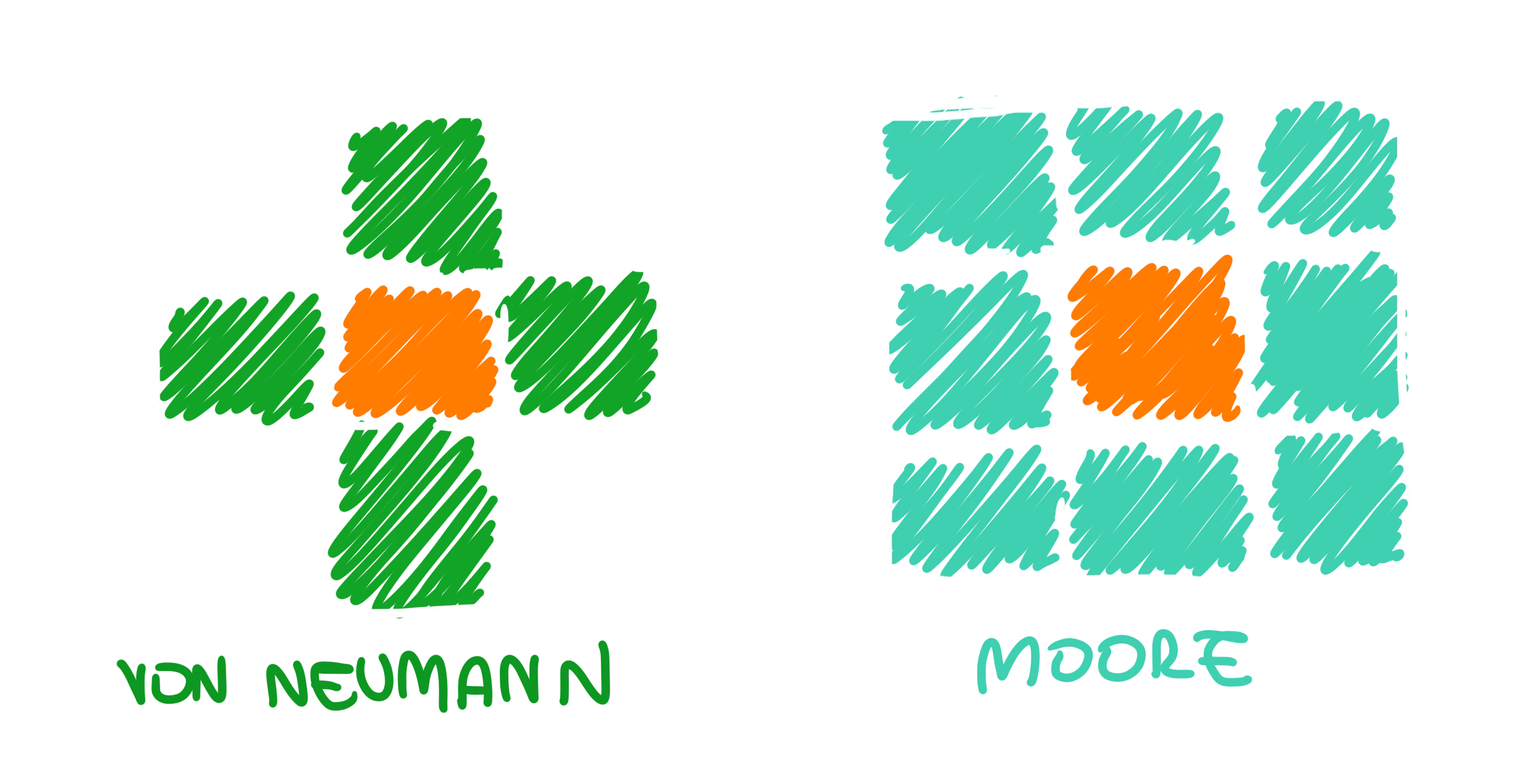
• 🏘️ While learning the theory about complex systems, we stated how the rules that regulate the agents' behaviour are defined through simple mechanisms and decisions based on the locality of the agents themselves. This locality is named neighbourhood and it is defined based on the world nature. For example, in a squared cells grid environment, the neighbourhood can be usually defined in two different ways: Von Neumann neighbourhood or Moore's neighbourhood. In AgentScript an agent provides the methods neighbors4 and neighbors to select respectively one of the two neighbourhoods.

• ⏭️ It is now time to give life to our model. The transition rule defines how the agent's state will change based on its neighbourhood. The nature of Game of Life's rules brings our attention to a sensitive aspect of ABM's programming. We can notice that the future of a cell is defined with respect to the number of living/dead neighbour cells. So, it will be crucial to update the cells altogether, based on the same previous state. That means avoiding updating, in the current step, the last cells from a mix of the previous step's state and already updated cells (at the end, the evaluation of all the cells is done through a for cycle). This kind of attention is often required while designing ABM's, cause different strategies while implementing the code will take us to different model evolutions. Now that this consideration has been done, we just need to follow the rules written above 🫡.

// ...

step() {
  // this is to "capture" the previous state for all the cells
  this.patches.ask((p) => {
    p.liveNeighbors = p.neighbors.with(
      (n) => n.breed === this.live
    ).length;
  });

  /**
  * Effective transition phase!
  * It could be written in a more elegant way. Left like
  * this to have a perfect match with what we wrote before.
  */
  this.patches.ask((p) => {
    if (p.breed === this.live && p.liveNeighbors < 2) {
      p.setBreed(this.dead);
      return;
    }

    if (
      p.breed === this.live &&
      (p.liveNeighbors === 2 || p.liveNeighbors === 3)
    ) {
      return;
    }

    if (p.breed === this.live && p.liveNeighbors > 3) {
      p.setBreed(this.dead);
    }

    if (p.breed === this.dead && p.liveNeighbors === 3) {
      p.setBreed(this.live);
    }
  });
}

// ...

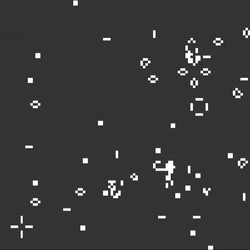
At this point, we just need to instantiate the View and the Animator to bring our model simulation to life.

Epidemic simulation

In the previous sections, we've built the basic knowledge needed to start building model simulations. In particular, we explored the framework and infrastructure required to set up the computational model. We are now ready to pick a complex system of our interest and throw it into this mechanism to start studying it. Before coding the actual (computational) agent, though, we need to model our system formally and analytically.

Epidemic Modeling

The design of the model I will present has started from the exploration of probably the most famous compartmental model used while studying infectious disease spreading: the SIR model. The idea of the SIR is that during a spread that occurs over time, people of a targeted population will be categorized into three main buckets:

• Susceptible (S): all the healthy individuals without immunity, hence at risk of getting infected. How the infection can spread is another design choice that we will address later.
• Infected (I): all the infected individuals. They can spread the disease.
• Recovered (R): when an individual recovers from the disease it becomes immune and will not be infected anymore.

Over time, individuals live their lives, getting in touch with each other and eventually spreading the disease around the population. In this basic setting, every individual typically progresses from susceptible to infectious to recovered, as often depicted by this kind of flow diagram:

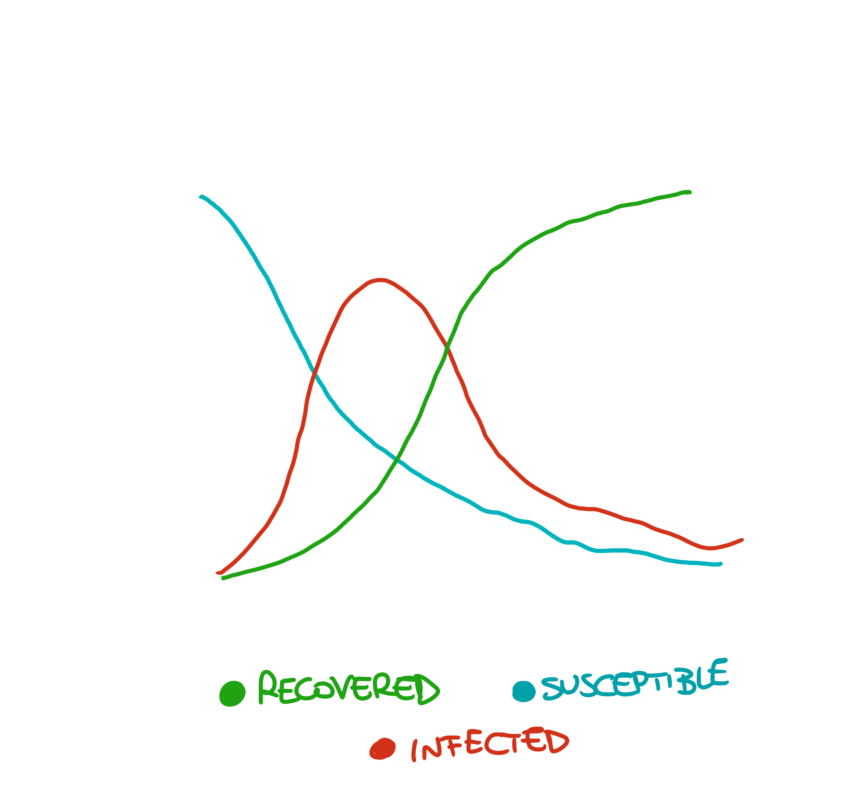
That is the core upon which I built my transition rule. Before diving into it, we need to understand how the environment has been defined. Starting from a city size (expressed as the number of cells squared, i.e., the area of our grid) a proportional number of families are generated:

• Each family has its own house, placed in the grid at random positions.
• Each family is composed of four individuals: two adults (35-50 y.o.), a youth (10-18 y.o.) and an aged individual (65-100 y.o.).
• The adults go to the office each morning at 8.00 am, coming back home at 6.00 pm.
• The youths go to school each morning at 8.00 am, coming back home at 4.00 pm.
• The aged ones stay at home, risking infection only through their family members.

At that point should be clear the two main ways in which the infection can spread:

• Individuals will visit common spaces in the city, such as cafes, buses, or stores while returning home or arriving at the office (or school, for that matter). In particular, an infected individual that goes through a cell will leave a certain amount of viral load that can affect other individuals going through that cell. The viral load will fade over time.
• Infected individuals can spread the infection to their family members due to the longer time they will spend together at home.

Note that, at the beginning of the simulation an outbreak is present to initialize a portion of the population as already infected.

We can now move on to diving deep into how the transition rule is structured. The last thing to keep in mind is that simulation allows for the definition of a user-defined virus, customizable through the choice of a set of parameters. The core of the model is a variation of the classical SIR model, namely a SEIRD model, defined as depicted below:

• Intro: as already said, the population will suffer from a starting outbreak of people infected and asymptomatic. In this way, we are sure that no individual will die prematurely without the chance of effectively spreading the infection (only symptomatic individuals can die). Furthermore, the chance of applying a lockdown strategy has been added: this will affect only symptomatic individuals. For that reason, the outbreak population is made up only by asymptomatic ones.
• A. Moving from Susceptible to Exposed: The infected individuals will go around the city, leaving a certain amount of viral load upon the different visited grid cells. Susceptible individuals will then happen to be on those cells, where they risk becoming Exposed with a certain probability computed as follows.
  $P_e = 1 - exp(-P_{infection} \cdot v_{load} \cdot k)$
  • $P_{infection}$

    is the probability of getting infected by this virus (hence, it is a virus-dependent parameter),
  • $v_{load}$

    is the amount of viral load left in the cell of interest. Note that multiple infected individuals can move across the same cell, contributing in summing up their viral loads.
  • $k$

    is just a scale factor, tunable to control and evaluate the realism of the simulation. From a mathematical point of view, it controls how steep is the exponential curve.
• B. Moving from Exposed to Infected: this step is time-based. After

  $T_{incubation}$

  days the Exposed individual will become Infected. At this point, it can be sick with or without symptoms with a probability

  $P_{symptoms}$

  . Both

  $T_{incubation}$

  and

  $P_{symptoms}$

  are virus-defined parameters.
• C. Healing from infection: a sick individual will return healthy with a probability that is directly proportional to the time it has been infected (with respect to another virus-defined parameter that indicates the average time of infection). Formally, this probability is computed as follows.
  $P_{heal} = \frac{1}{1 + exp(-k \cdot \Delta T )}$
  • $\Delta T$

    is computed as the difference (in days) between the duration of the individual infection and the average duration of the infection (

    $T_{disease}$

    ).
  • $k$

    is again a scale factor. The idea of the former probability is to increase when approacching toward the average time of the disease. This scalar controls how steep the curve is toward this value.
  Now, if the individual will heal, it may become Immune with a probability

  $P_{immune}$

  . Otherwise, it will revert to susceptibility.
• Moving from Infected (symptomatic) to Death: while being infected and symptomatic, the individual has a chance of dying proportional to its age, the virus mortality

  $P_{mortality}$

  (expressed as probability as well) and the time has been sick.

That's it for the transition mechanism! To recap, those are the parameters that a virus should define to be tested inside this simulation:

• $P_{infection}$

  is the virus spread probability.
• $P_{symptoms}$

  is the probability of being symptomatic when infected.
• $P_{mortality}$

  is the virus mortalitiy probability.
• $P_{immunity}$

  is the probability of becoming immune to the virus after being healed.
• $T_{incubation}$

  is the time (in days) needed to become infected after being exposed.
• $T_{disease}$

  is the average time (in days) of the disease duration.

To finish the model, two containment measures are configurable:

• Lockdown: when an individual is infected and symptomatic, once at home (it could be infected outside) it will not go out anymore until recovery. The Lockdown setting is expressed as a percentage of people that will respect it and is tunable before starting the simulation.
• Mask usage: when an individual is infected and symptomatic, will use the mask to protect other individuals against him. Practically, an infected individual with a mask on will leave half of the viral load onto the cells. The mask usage setting is expressed as a percentage of people that will decide to use it and is tunable before starting the simulation.

Viral Verse (the actual simulator)

All the theories discussed have been implemented in a simple web application to give users a customizable simulation of an infection spread. The starting point is the definition of a user-defined virus (configurable with the parameters listed before). Furthermore, some environment settings can be modified (e.g., city area, mask usage or lockdown percentage).

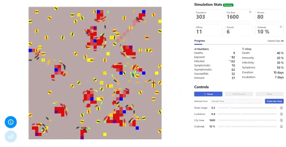
Once the simulation is started, it is possible to investigate the evolution of the different SIR curves of the current run.

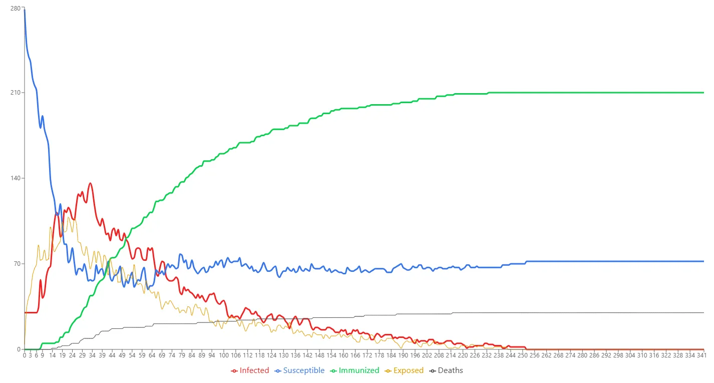
You can find the source code on GitHub. Any contribution will be more than appreciated. 😄

📚 References

• Think Complexity (Allen B. Downey)
• Compartmental Models in Epidemiology

💻 Practical References:

• AgentScript